12. Case Study: Autodiff
Today, we will talk about another case study on automatic differentiation (autodiff), while avoiding some of the complex mathematical concepts.
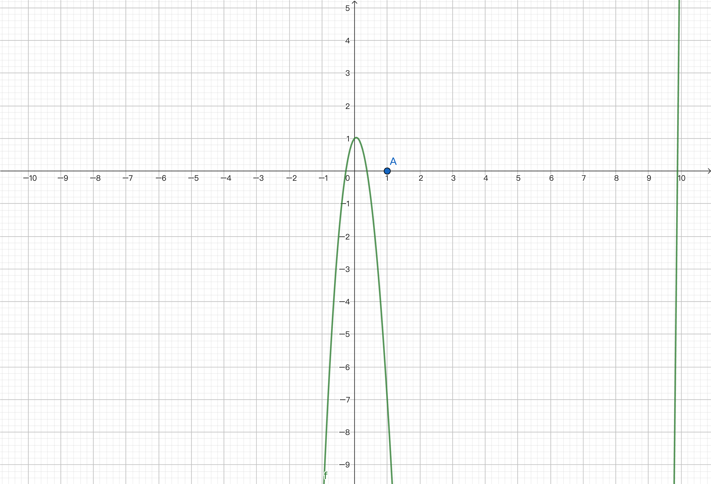
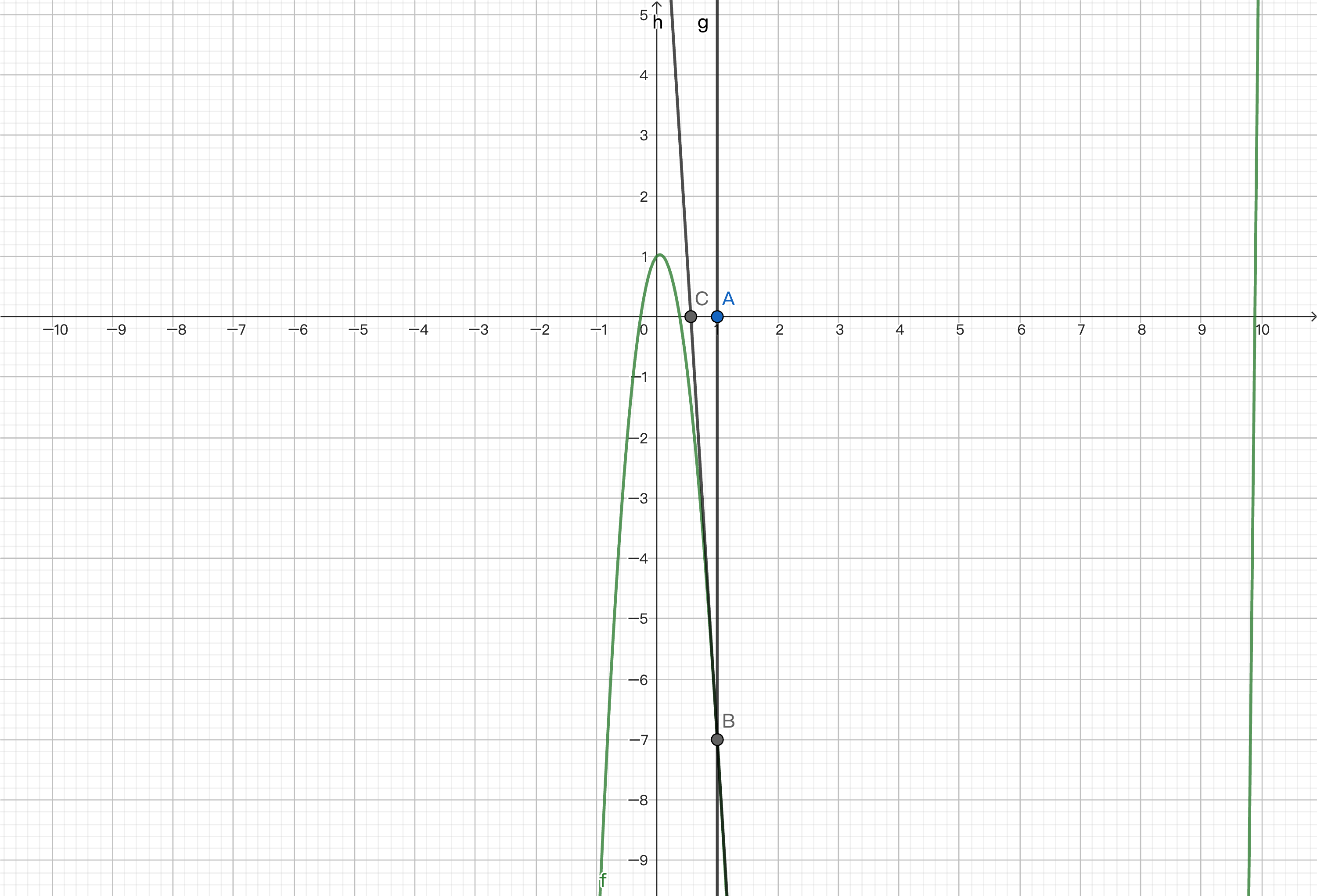
Differentiation is an important operation in computer science. In machine learning, neural networks based on gradient descent apply differentiation to find local minima for training. You might be more familiar with solving functions and approximating zeros using Newton's method. Let's briefly review it. Here, we have plotted a function and set the initial value to 1, which is point A on the number axis.
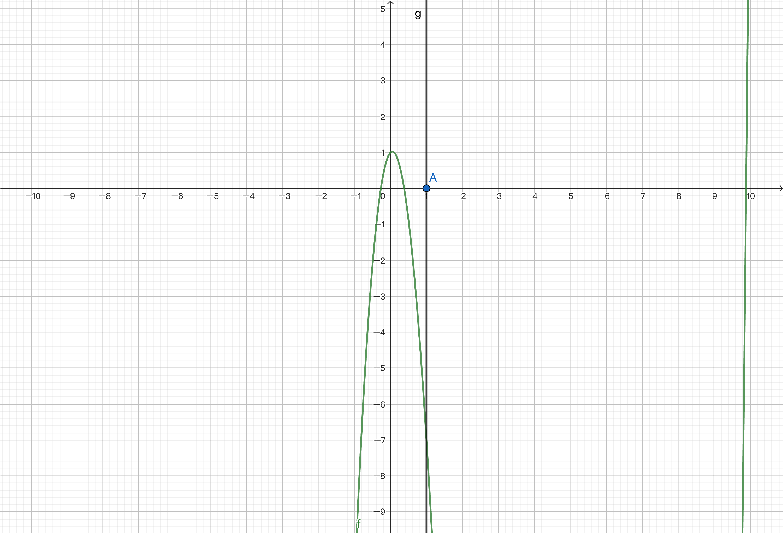
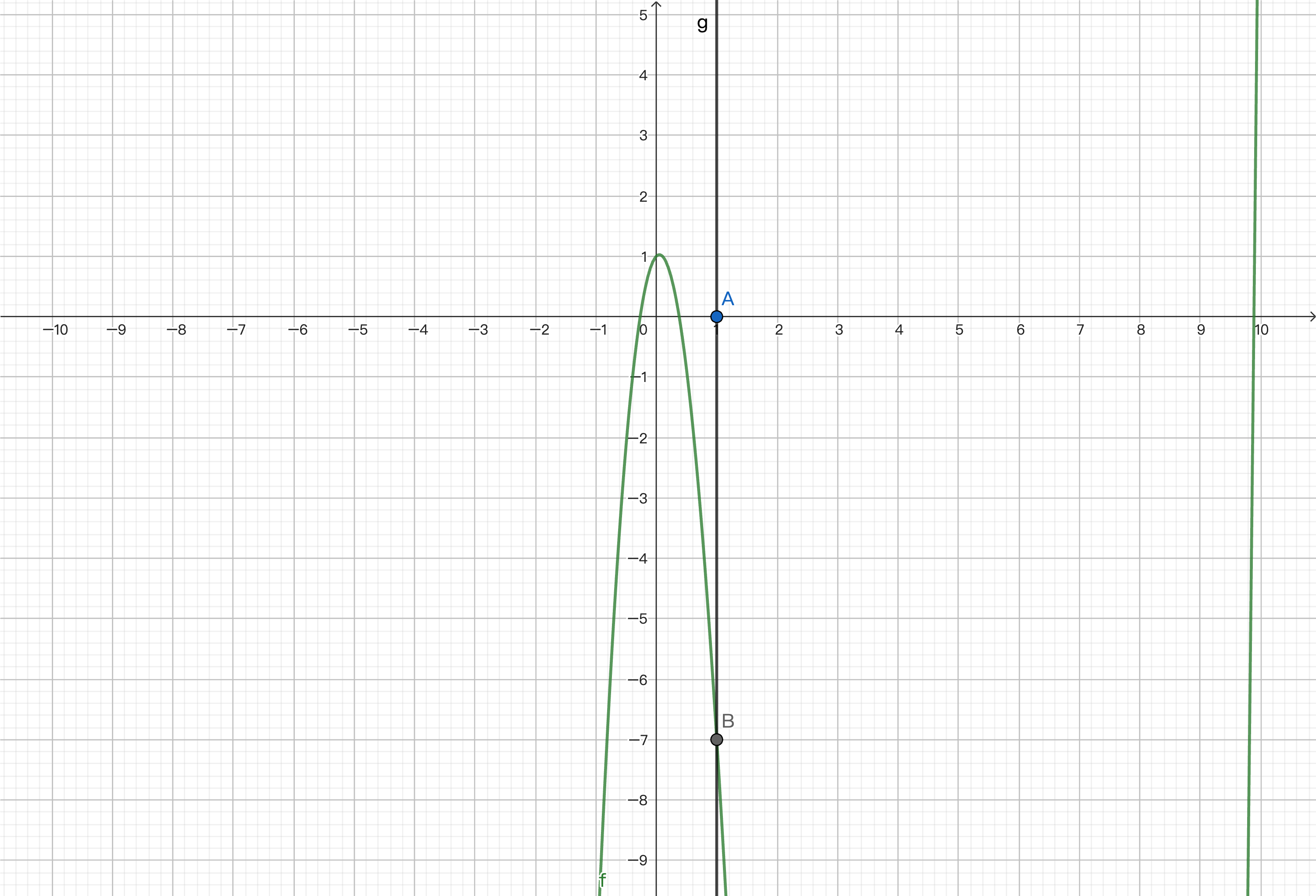
We want to approximate the zeros near it. We calculate point B on the function corresponding to the x-coordinate of this point and find the derivative at the point, which is the slope of the tangent line at that point.
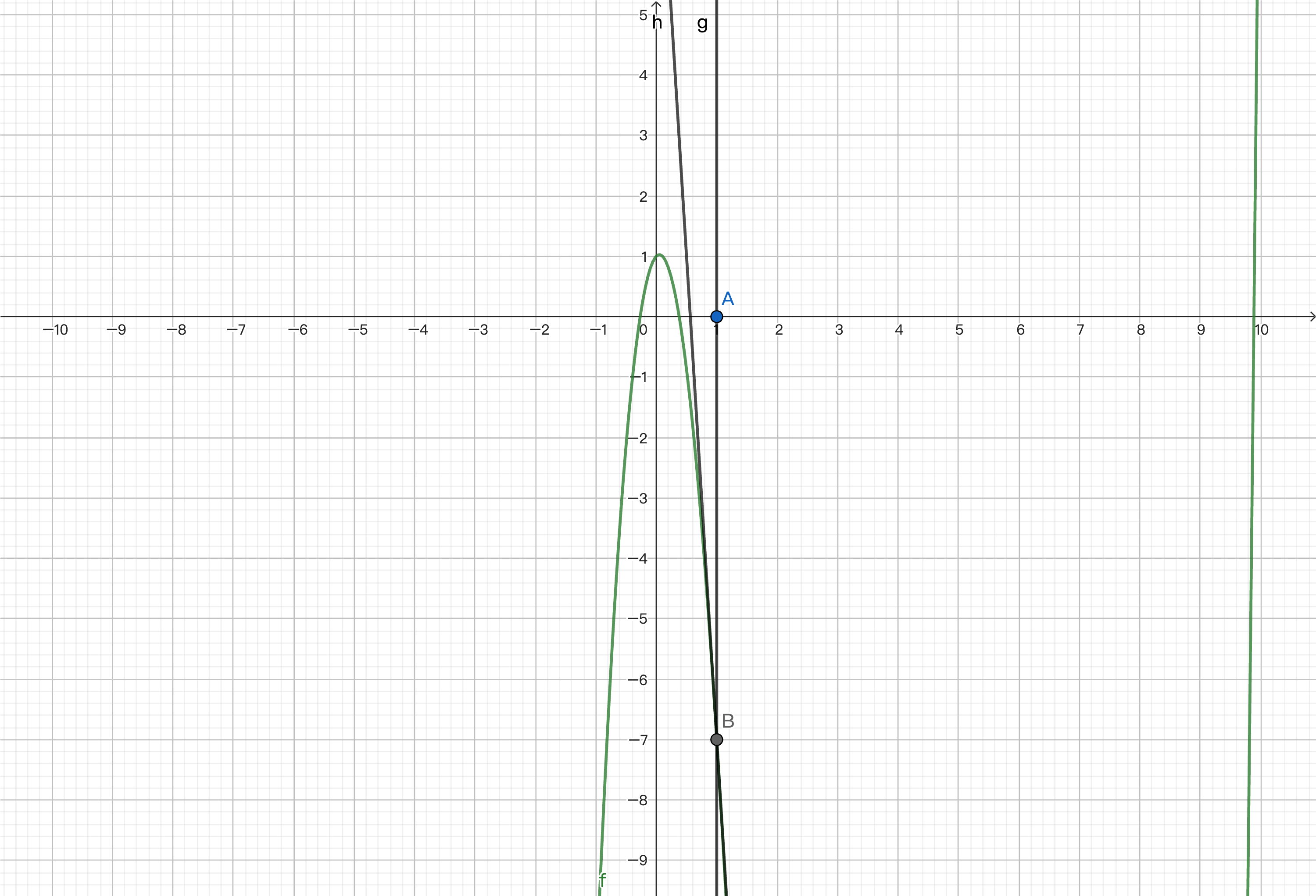
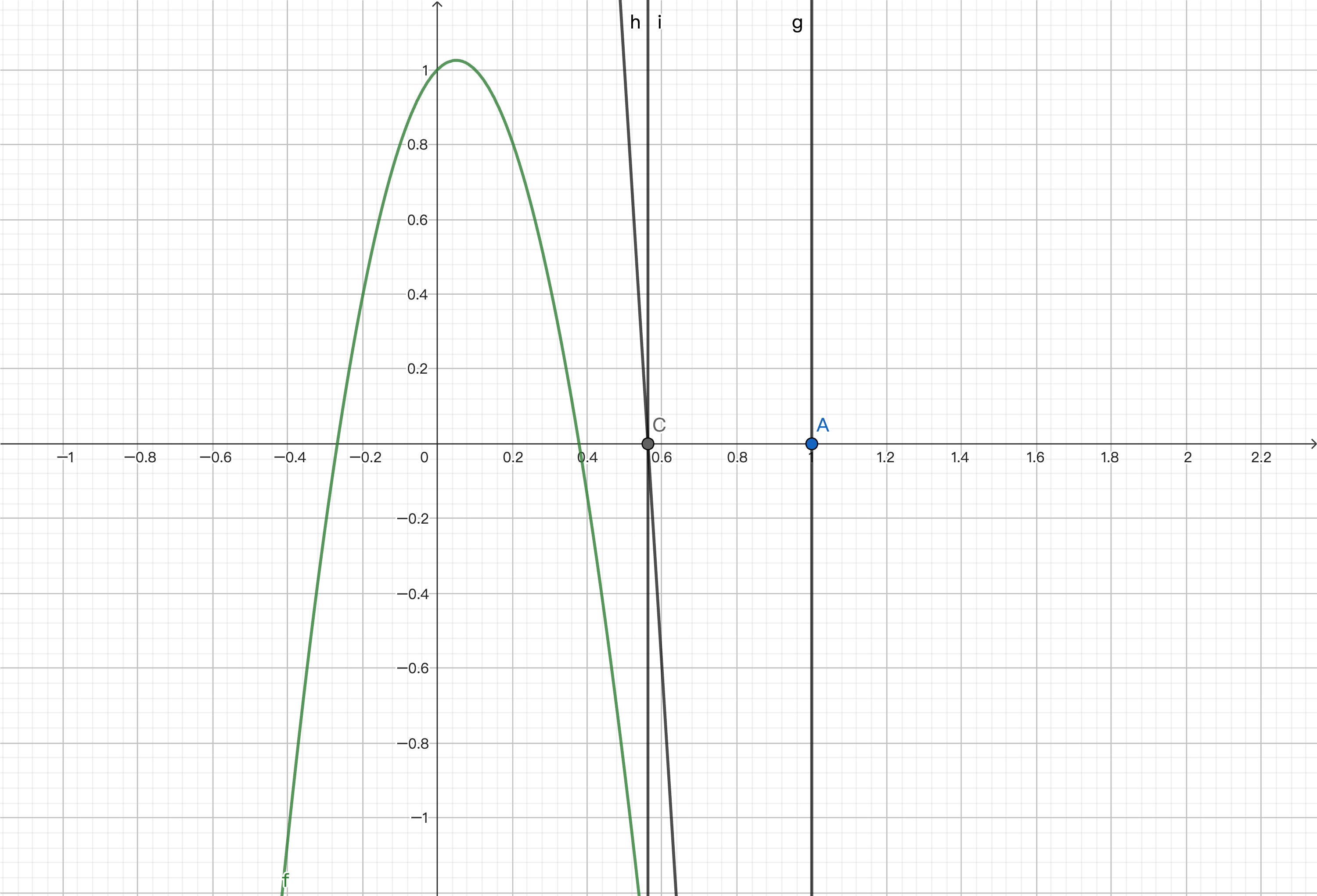
By finding the intersection of the tangent line and the x-axis, we get a value that approximates zero.
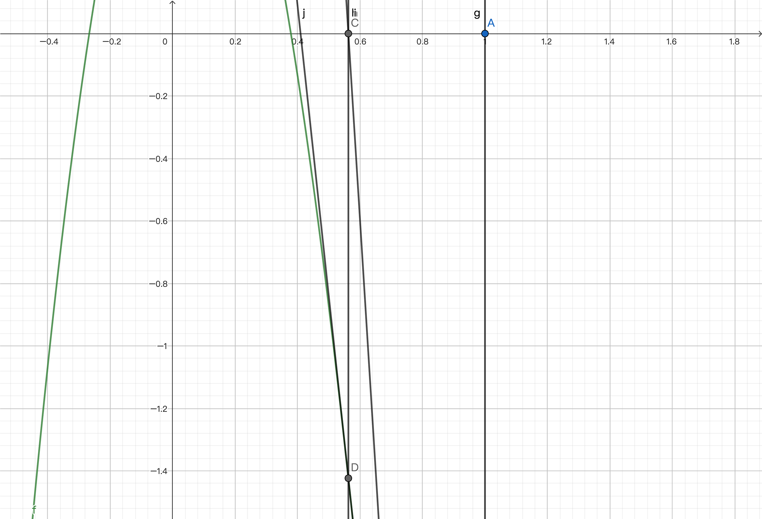
We then repeat the process to find the point corresponding to the function, calculate the derivative, and find the intersection of the tangent line and the x-axis.
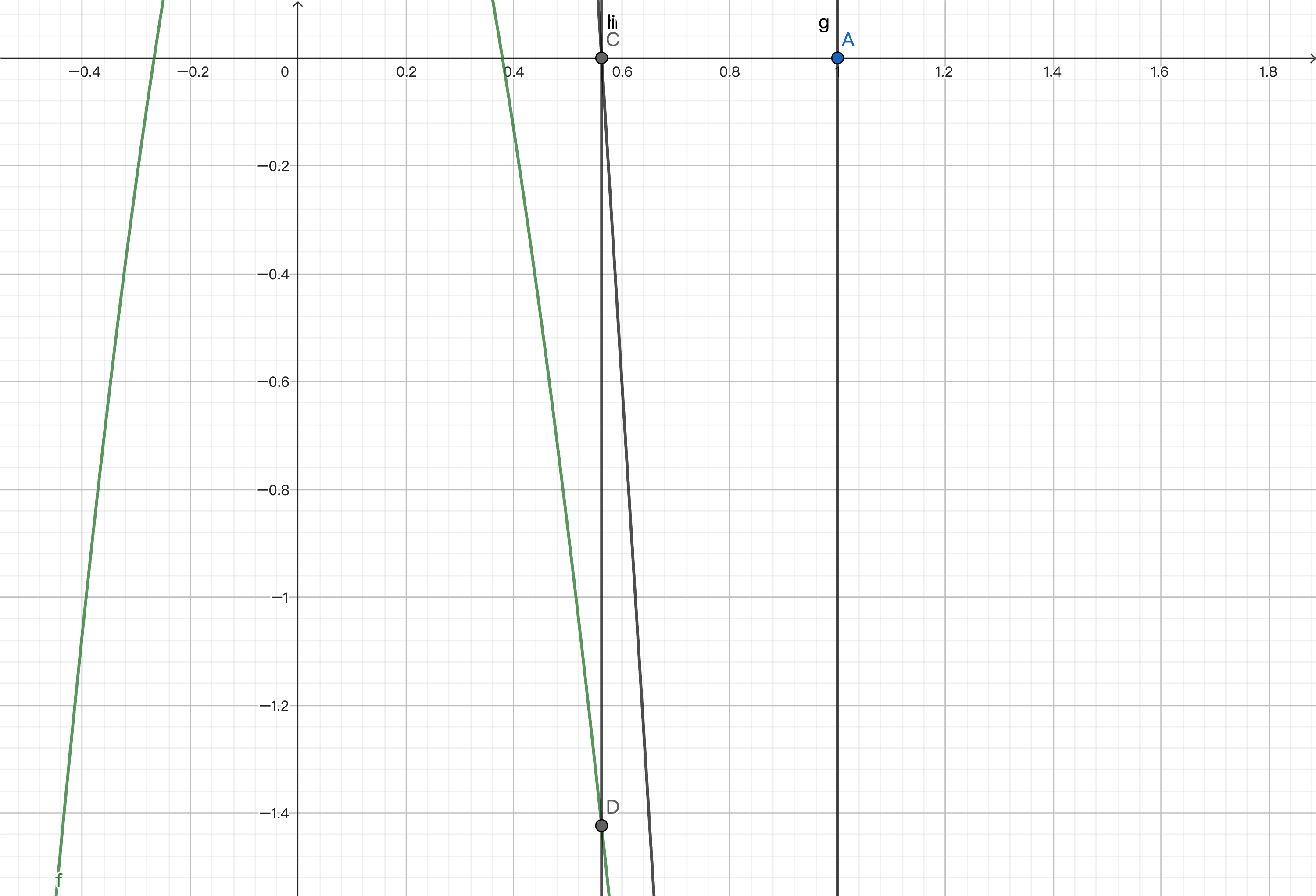
This way, we can gradually approach zero and get an approximate solution. We will provide the code implementation at the end.
Today, we will look at the following simple combination of functions, involving only addition and multiplication. For example, when calculating 5 times
Example:
Differentiation
There are several ways to differentiate a function. The first method is manual differentiation where we use a piece of paper and a pen as a natural calculator. The drawback is that it's easy to make mistakes with complex expressions and we can't just manually calculate 24 hours a day. The second method is numerical differentiation:
// Need to define additional native operators for the same effect
fn max[N : Number](x : N, y : N) -> N {
 if x.value() > y.value() { x } else { y }
}
Lastly, the fourth method is automatic differentiation. Automatic differentiation uses the derivative rules of composite functions to perform calculation and differentiation by combining basic operations, which also aligns with modular thinking. Automatic differentiation is divided into forward and backward differentiation. We will introduce them one by one.
Symbolic Differentiation
Let's first look at symbolic differentiation. We define expressions using an enum type. An expression can be a constant, a variable indexed starting from zero, or the sum or product of two functions. Here we define simple constructors and overload operators to produce more concise expressions. Finally, in line 15, we use pattern matching to define a method that computes function values based on symbols, with the input being a vector (omitted here).
enum Symbol {
  Constant(Double)
  Var(Int)
  Add(Symbol, Symbol)
  Mul(Symbol, Symbol)
} derive(Show)

// Define simple constructors and overload operators
fn Symbol::constant(d : Double) -> Symbol { Constant(d) }
fn Symbol::var(i : Int) -> Symbol { Var(i) }
fn Symbol::op_add(f1 : Symbol, f2 : Symbol) -> Symbol { Add(f1, f2) }
fn Symbol::op_mul(f1 : Symbol, f2 : Symbol) -> Symbol { Mul(f1, f2) }

// Compute function values
fn Symbol::compute(self : Symbol, input : Array[Double]) -> Double {
  match self {
    Constant(d) => d
    Var(i) => input[i] // get value following index
    Add(f1, f2) => f1.compute(input) + f2.compute(input)
    Mul(f1, f2) => f1.compute(input) * f2.compute(input)
    }
}
Let's review the derivative rules for any constant function, any variable partially differentiated with respect to itself, the sum of two functions and the product of two functions. For example, the derivative of
if is a constant function
We'll use the previous definition to construct our example function. As we can see, the multiplication and addition operations look very natural because MoonBit allows us to overload some operators.
fn differentiate(self : Symbol, val : Int) -> Symbol {
  match self {
      Constant(_) => Constant(0.0)
    Var(i) => if i == val { Constant(1.0) } else { Constant(0.0) }
    Add(f1, f2) => f1.differentiate(val) + f2.differentiate(val)
    Mul(f1, f2) => f1 * f2.differentiate(val) + f1.differentiate(val) * f2
  }
}
After constructing the expression, we differentiate it to get the corresponding expression, as shown in line 7 and then compute the partial derivative based on the input. Without simplification, the derivative expression we obtain might be quite complicated, as shown below.
fn example() -> Symbol {
  Symbol::constant(5.0) * Symbol::var(0) * Symbol::var(0) + Symbol::var(1)
}

test "Symbolic differentiation" {
  let input : Array[Double] = [10.0, 100.0]
  let symbol : Symbol = example() // Abstract syntax tree of the function
  assert_eq!(symbol.compute(input), 600.0)
  // Expression of df/dx
  inspect!(symbol.differentiate(0),
  content="Add(Add(Mul(Mul(Constant(5.0), Var(0)), Constant(1.0)), Mul(Add(Mul(Constant(5.0), Constant(1.0)), Mul(Constant(0.0), Var(0))), Var(0))), Constant(0.0))")
  assert_eq!(symbol.differentiate(0).compute(input), 100.0)
}
Of course, we can define some simplification functions or modify the constructors to simplify the functions. For example, we may simplify the result of addition. Adding 0 to any number is still that number, so we can just keep the number; and when adding two numbers, we can simplify them before computing with other variables. Lastly, if there's an integer on the right, we can move it to the left to avoid writing each optimization rule twice.
fn Symbol::op_add_simplified(f1 : Symbol, f2 : Symbol) -> Symbol {
  match (f1, f2) {
    (Constant(0.0), a) => a
      (Constant(a), Constant(b)) => Constant(a + b)
      (a, Constant(_) as const) => const + a
      (Mul(n, Var(x1)), Mul(m, Var(x2))) =>
        if x1 == x2 {
          Mul(m + n, Var(x1))
        } else {
          Add(f1, f2)
        }
      _ => Add(f1, f2)
  } }
Similarly, we can simplify multiplication. Multiplying 0 by any number is still 0, multiplying 1 by any number is still the number itself, and we can simplify multiplying two numbers, etc.
fn Symbol::op_mul_simplified(f1 : Symbol, f2 : Symbol) -> Symbol {
  match (f1, f2) {
    (Constant(0.0), _) => Constant(0.0) // 0 * a = 0
    (Constant(1.0), a) => a             // 1 * a = 1
    (Constant(a), Constant(b)) => Constant(a * b)
    (a, Constant(_) as const) => const * a
    _ => Mul(f1, f2)
  } }
After such simplifications, we get a more concise result. Of course, our example is relatively simple. In practice, more simplification is needed, such as combining like terms, etc.
let diff_0_simplified : Symbol = Mul(Constant(5.0), Var(0))
Automatic Differentiation
Now, let's take a look at automatic differentiation. We first define the operations we want to implement through an interface, which includes constant constructor, addition, and multiplication. We also want to get the value of the current computation.
trait Number  {
  constant(Double) -> Self
  op_add(Self, Self) -> Self
  op_mul(Self, Self) -> Self
  value(Self) -> Double // Get the value of the current computation
}
With this interface, we can use the native control flow of the language for computation and dynamically generate computation graphs. In the following example, we can choose an expression to compute based on the current value of
fn max[N : Number](x : N, y : N) -> N {
  if x.value() > y.value() { x } else { y }
}

fn relu[N : Number](x : N) -> N {
max(x, N::constant(0.0))
}
Forward Differentiation
We will start with forward differentiation. It is relatively straightforward that it directly uses the derivative rules to simultaneously calculate dual number in linear algebra. You are encouraged to dive deeper into it if you find it interesting. Let's construct a struct containing dual numbers, with one field being the value of the current node and the other being the derivative of the current node. It is very simple to construct from constants: the value is the constant, and the derivative is zero. It is also very straightforward to get the current value where we just access the corresponding variable. Here we add a helper function. For a variable, besides its value, we also need to determine if it is the variable to differentiate, and if so, its derivative is 1, otherwise, it is 0, as previously explained.
struct Forward {
  value : Double      // Current node value f
  derivative : Double // Current node derivative f'
} derive(Show)

fn Forward::constant(d : Double) -> Forward { { value: d, derivative: 0.0 } }
fn Forward::value(f : Forward) -> Double { f.value }

// determine if to differentiate the current variable
fn Forward::var(d : Double, diff : Bool) -> Forward {
  { value : d, derivative : if diff { 1.0 } else { 0.0 } }
}
Next, let's define methods for addition and multiplication, using the derivative rules to directly calculate derivatives. For example, the value of the sum of two functions
fn Forward::op_add(f : Forward, g : Forward) -> Forward { {
  value : f.value + g.value,
  derivative : f.derivative + g.derivative // f' + g'
} }

fn Forward::op_mul(f : Forward, g : Forward) -> Forward { {
  value : f.value * g.value,
  derivative : f.value * g.derivative + g.value * f.derivative // f * g' + g * f'
} }
Finally, we use the previously defined example with conditionals to calculate derivatives. Note that forward differentiation can only compute the derivative with respect to one input parameter at a time, making it suitable for cases where there are more output parameters than input parameters. In neural networks, however, we typically have a large number of input parameters and one output. Therefore, we need to use the backward differentiation introduced next.
test "Forward differentiation" {
// Forward differentiation with abstraction
  inspect!(relu(Forward::var(10.0, true)), content="{value: 10.0, derivative: 1.0}")
  inspect!(relu(Forward::var(-10.0, true)), content="{value: 0.0, derivative: 0.0}")
// f(x, y) = x * y => df/dy(10, 100)
  inspect!(Forward::var(10.0, false) * Forward::var(100.0, true), ~content="{value: 1000.0, derivative: 10.0}")
}
Backward Differentiation
Backward differentiation utilizes the chain rule for calculation. Suppose we have a function
- Given
For example, for
- Example:
- Decomposition:
- Differentiation:
- Combination:
- Decomposition:
Here we demonstrate an implementation in MoonBit. The backward differentiation node consists of the value of the current node and a function named backward. The backward function uses the accumulated derivatives from the result to the current node (the parameters) to update the derivatives of all parameters that construct the current node. For example, below, we define a node that represents the input. We use a Ref to accumulate the derivatives calculated along all paths. When the backward computation process reaches the end, we add the partial derivative of the function with respect to the current variable to the accumulator. This partial derivative is just the partial derivative of one path in the computation graph. As for constants, they have no input parameters, so the backward function does nothing.
struct Backward {
  value : Double              // Current node value
  backward : (Double) -> Unit // Update the partial derivative of the current path
} derive(Show)

fn Backward::var(value : Double, diff : Ref[Double]) -> Backward {
  // Update the partial derivative along a computation path df / dvi * dvi / dx
  { value, backward: fn { d => diff.val = diff.val + d } }
}

fn Backward::constant(d : Double) -> Backward {
  { value: d, backward: fn { _ => () } }
}

fn Backward::backward(b : Backward, d : Double) -> Unit { (b.backward)(d) }

fn Backward::value(backward : Backward) -> Double { backward.value }
Next, let's look at addition and multiplication. Suppose the functions backward function. So we can see in line 4 that the parameter we pass to
fn Backward::op_add(g : Backward, h : Backward) -> Backward {
  {
    value: g.value + h.value,
    backward: fn(diff) { g.backward(diff * 1.0); h.backward(diff * 1.0) },
  }
}

fn Backward::op_mul(g : Backward, h : Backward) -> Backward {
  {
    value: g.value * h.value,
    backward: fn(diff) { g.backward(diff * h.value); h.backward(diff * g.value) },
  }
}
Lastly, we'll see how to use it. Let's construct two Refs to store the derivatives of 1.0 corresponds to the derivative of Refs are updated, and we can obtain the derivatives of all input parameters simultaneously.
test "Backward differentiation" {
  let diff_x = Ref::{ val: 0.0 } // Store the derivative of x
  let diff_y = Ref::{ val: 0.0 } // Store the derivative of y
  let x = Backward::var(10.0, diff_x)
  let y = Backward::var(100.0, diff_y)
  (x * y).backward(1.0) // df / df = 1
  inspect!(diff_x, content="{val: 100.0}")
  inspect!(diff_y, content="{val: 10.0}")
}
Now with backward differentiation, we can try to write a neural network. In this lecture, we'll only demonstrate automatic differentiation and Newton's method to approximate zeros. Let's use the interface to define the functions we saw at the beginning.
Then, we'll use Newton's method to find the value. Since there is only one parameter, we'll use forward differentiation.
-
fn example_newton[N : Number](x : N) -> N {
  x * x * x + N::constant(-10.0) * x * x + x + N::constant(1.0)
}
To approximate zeros with Newton's method:
- First, define
as the iteration variable with an initial value of 1.0. Since is the variable with respect to which we are differentiating, we'll set the second parameter to be true. - Second, define an infinite loop.
- Third, in line 5, compute the value and derivative of the function corresponding to
. - Fourth, in line 6, if the value divided by the derivative (i.e., the step size we want to approximate) is small enough, it indicates that we are very close to zero, and we terminate the loop.
- Last, in line 7, if the condition is not met, update the value of
to be the previous value minus the value divided by the derivative and then continue the loop.
In this way, we iterate through the loop to eventually get an approximate solution.
test "Newton's method" {
  (loop Forward::var(1.0, true) { // initial value
    x => {
      let { value, derivative } = example_newton(x)
      if (value / derivative).abs() < 1.0e-9 {
        break x.value // end the loop and have x.value as the value of the loop body
      }
      continue Forward::var(x.value - value / derivative, true)
    }
  } |> assert_eq!(0.37851665401644224))
}
Summary
To summarize, in this lecture we introduced the concept of automatic differentiation. We presented symbolic differentiation and two different implementations of automatic differentiation. For students interested in learning more, we recommend the 3Blue1Brown series on deep learning (including topics like gradient descent, backpropagation algorithms), and try to write your own neural network.