13. Case Study: Neural Network
The aim of this chapter is to manually implement a gradient descent-based neural network using the automatic differentiation technique introduced in Chapter 12.
In this chapter, we will be using the Iris dataset, which is considered the "Hello World" of machine learning. It was first released in 1936 and contains 3 classes with 50 samples each, representing different types of iris plants. Each sample comprises 4 features: sepal length, sepal width, petal length, and petal width. Our task is to develop and train a neural network to accurately classify the type of an iris plant based on its features, with an accuracy rate of over 95%.
Typically, it is important to first examine and understand the dataset before implementing and training an machine learning model. However, since our main subject in this chapter is to implement a neural network, we will skip this step.
Machine learning is a vast and complex field, and the knowledge related to neural networks is particularly intricate. Therefore, the content we cover here is just a brief introduction, and we will only showcase a portion of the code. If you are interested, you can find the complete code here.
The Structure of a Neural Network
Neural networks are a subtype of machine learning. As the name suggests, they simulate the neural structure of the human brain. A classic neural network usually consists of multiple layers and interconnected neurons. A neuron typically has multiple inputs, a single output, and weights to calculate the output signal based on the input signals. A neuron typically activates once it reaches a certain threshold.
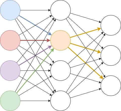
The above diagram an illustration of a neural network. Each node represents a neuron. The yellow neuron receives inputs from the four neurons in the left layer and passes its output to the neurons in the right layer.
A classic neural network typically consists of an input layer, an output layer, and one or more hidden layers in between. The input layer receives the input values, while the output layer provides the computed results. As for the hidden layers, if the number of hidden layers becomes large, the network can be called a deep neural network.
The structure of a neural network includes the number of hidden layers, the number of neurons in each layer, and the connectivity between layers and neurons. For example, in a feedforward neural network, the connections between neurons do not form cycles. The activation function of neurons is also one of the hyperparameters of the neural network. Each of these parameter choices can be a complex topic on its own.
The network we just saw is quite suitable for our task. The input layer has four neurons, each corresponding to a feature. The output layer has three neurons, each representing the likelihood of belonging to each type of iris. The final classification result depends on which likelihood is the highest. We chose the simplest structure, a fully connected feedforward neural network, where each neuron is connected to all neurons in the previous layer.
For each neuron, its output is based on a linear transformation of the inputs:
For the activation function in the hidden layers, we chose the Rectified Linear Unit (ReLU) function:
In the output layer, we chose to use the softmax function:
Implementation
The above is the entire structure of this neural network. Now, we will try to implement it with MoonBit.
Basic Operations
First, we define an abstraction for operations. The operations we need to perform include:
constant: type conversion fromDoubleto a certain type;value: retrieving the intermediate result from that type; andop_add,op_neg,op_mul,op_div,exp: addition, multiplication, division, negation, and exponential operations.
The types that conform to these operations include Double itself, as well as other types that we may use in automatic differentiation.
trait Base {
  constant(Double) -> Self
  value(Self) -> Double
  op_add(Self, Self) -> Self
  op_neg(Self) -> Self
  op_mul(Self, Self) -> Self
  op_div(Self, Self) -> Self
  exp(Self) -> Self // for computing softmax
}
Activation Function
Next, let's talk about the activation functions. The implementation of ReLU is straightforward. We can simply check whether the current computed value is positive or negative.
fn reLU[T : Base](t : T) -> T {
  if t.value() < 0.0 {
    T::constant(0.0)
  } else {
    t
  }
}
As for the softmax function, we start by creating an array to store the output probabilities, with all values initialized to
fn softmax[T : Base](inputs : Array[T]) -> Array[T] {
  let n = inputs.length()
  let outputs : Array[T] = Array::make(n, T::constant(0.0))
  let mut sum = T::constant(0.0)
  for i = 0; i < n; i = i + 1 {
    sum = sum + inputs[i].exp()
  }
  for i = 0; i < n; i = i + 1 {
    outputs[i] = inputs[i].exp() / sum
  }
  outputs
}
Input Layer → Hidden Layer
Next, let's implement the forward propagation function from the input layer to the hidden layer. We iterate over each parameter |> to obtain the final output.
fn input2hidden[T : Base](inputs: Array[Double], param: Array[Array[T]]) -> Array[T] {
  let outputs : Array[T] = Array::make(param.length(), T::constant(0.0))
  for output = 0; output < param.length(); output = output + 1 { // 4 outputs
    for input = 0; input < inputs.length(); input = input + 1 { // 4 inputs
      outputs[output] = outputs[output] + T::constant(inputs[input]) * param[output][input]
    }
    outputs[output] = outputs[output] + param[output][inputs.length()] |> reLU // constant
  }
  outputs
}
Hidden Layer → Output Layer
The function from the hidden layer to the output layer is basically the same. The only change is that we replaced the ReLU function with a softmax function.
fn hidden2output[T : Base](inputs: Array[T], param: Array[Array[T]]) -> Array[T] {
  let outputs : Array[T] = Array::make(param.length(), T::constant(0.0))
  for output = 0; output < param.length(); output = output + 1 { // 3 outputs
    for input = 0; input < inputs.length(); input = input + 1 { // 4 inputs
      outputs[output] = outputs[output] + inputs[input] * param[output][input]
    }
    outputs[output] = outputs[output] + param[output][inputs.length()] // constant
  }
  outputs |> softmax
}
Now, we have successfully implemented a neural network. We can use its parameters to classify any sample. Therefore, we only have one final task to do, which is to determine the value of the parameters.
Training
No one can know the best parameters in advance. They need to be obtained through training. The training of neural networks is generally divided into 3 steps:
- We need a cost function to tell us the "distance" between the current result and the expected result. Here, since we are dealing with a multi-classification problem, we use cross-entropy as the cost function.
- In order to know how to adjust parameters to minimize cost, we use the gradient descent method. That is, we will compute the partial derivative of each parameter, and adjust the parameters in the opposite direction.
- In addition to the direction of adjustment, we also need to determine the amplitude of each adjustment. This can be determined by the learning rate, which itself can also be adjusted through various strategies, and we choose exponential decay here.
Let's introduce and implement them one by one.
Cost Function
There is no unified cost function in the world because different machine learning tasks have different goals. For a multi-classification problem, cross-entropy is a typical choice:
We can explain the formula this way: for a classification, the ideal result should be 100%, but the result we obtained with our current parameters is
trait Log {
  log(Self) -> Self // for computing cross-entropy
}
fn cross_entropy[T : Base + Log](inputs: Array[T], expected: Int) -> T {
  -inputs[expected].log()
}
Gradient Descent
With the cost function in place, the next step is to perform gradient descent through backpropagation. Since we already covered this in Chapter 12, we will simply show the code here.
Accumulate the partial derivatives:
fn Backward::param(param: Array[Array[Double]], diff: Array[Array[Double]],
  i: Int, j: Int) -> Backward {
  {
    value: param[i][j],
    propagate: fn() {  },
    backward: fn { d => diff[i][j] = diff[i][j] + d}
  }
}
Compute the cost and perform backward differentiation accordingly:
fn diff(inputs: Array[Double], expected: Int,
    param_hidden: Array[Array[Backward]], param_output: Array[Array[Backward]]) -> Unit {
  let result = inputs
    |> input2hidden(param_hidden)
    |> hidden2output(param_output)
    |> cross_entropy(expected)
  result.backward(1.0)
}
Adjust parameters based on the gradients:
fn update(params: Array[Array[Double]],
          diff: Array[Array[Double]], step: Double) -> Unit {
  for i = 0; i < params.length(); i = i + 1 {
    for j = 0; j < params[i].length(); j = j + 1 {
      params[i][j] = params[i][j] - step * diff[i][j]
    }
  }
}
Learning Rate
Next, we need to adjust the learning rate. An inappropriate learning rate can cause worse performance, or even failure to converge to the optimal result.
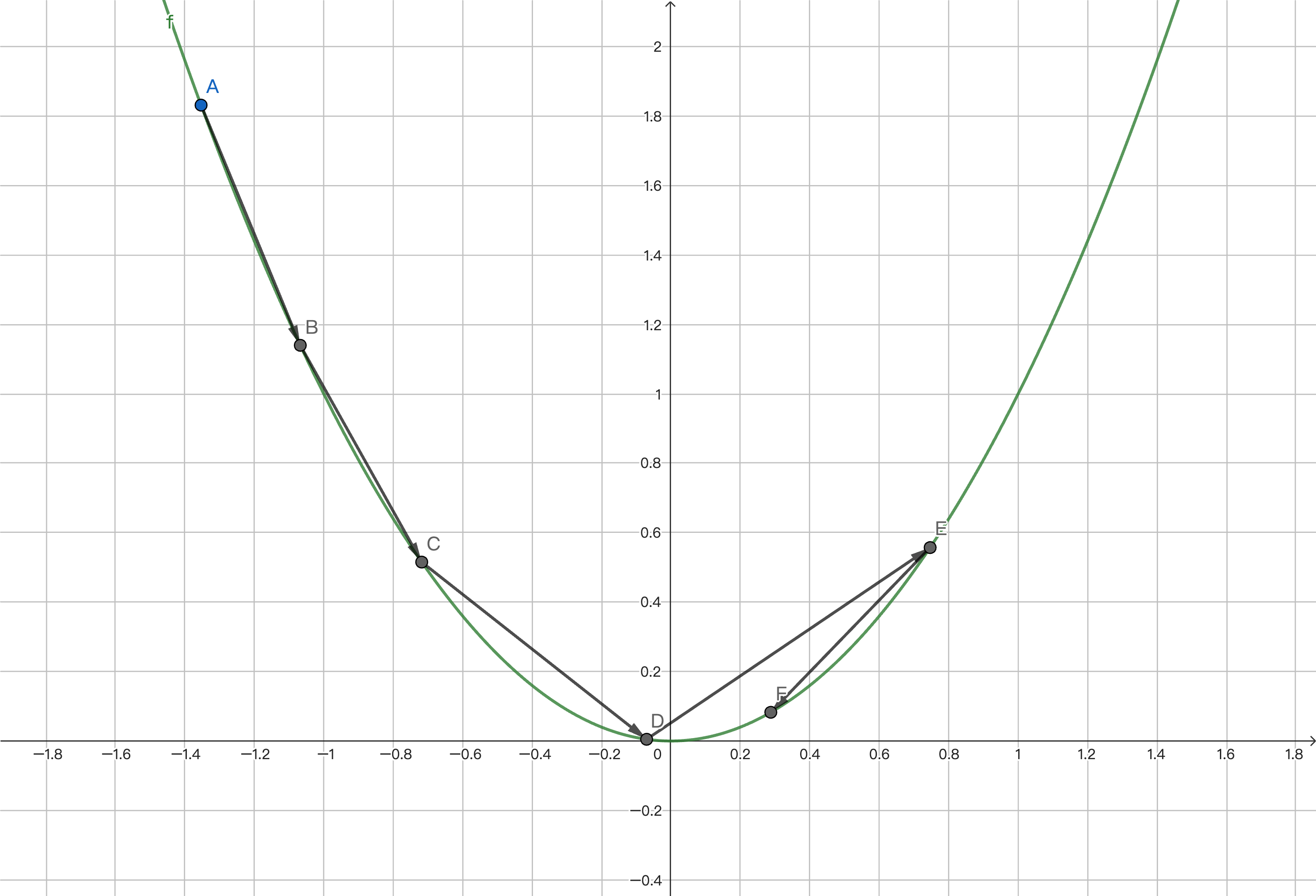
The figure above is just a conceptual example and does not correspond to our specific scenario.
If we want to find the lowest point of a function, which is where the cost function is minimized, we continuously approach it by taking derivatives and moving the corresponding step size. However, if the step size remains constant, we will overshoot the lowest point, then return and overshoot it again, oscillating below it and unable to converge. Therefore, we choose exponential decay for the learning rate here:
That is to say, the learning rate gradually decreases as the number of training epochs increases, achieving a fast approach in the initial stage and a gradual approach in the final stage.
Training and Testing
Finally, we can use the data to train our neural network. Usually, we need to randomly divide the dataset into two parts: the training set and the testing set. During the training phase, we compute the cost function and perform differentiation based on the data from the training set, and adjust the parameters based on the learning rate. The testing set is used to evaluate the results after all the training is completed. This is to avoid overfitting, where the model performs well on the training set but fails on general cases. This is also why the data in the training set needs to be randomly split.
For example, if our complete dataset contains 3 types of iris flowers, and the training set only contains two types of iris flowers, the model will never be able to correctly identify the third type of iris flower. In our case, we have a relatively small amount of training data, so we can perform full batch training, meaning that each epoch consists of one iteration, in which all the training samples are used. However, if we have a larger amount of data, we may perform mini batch training instead by splitting an epoch into several iterations and select a subset of the training data for each iteration.
Summary
This chapter introduces the basics of neural networks, including the structure and the training process of a neural network. Although the content is not in-depth, it is enough to give you a preliminary understanding of the topic. If you are interested, you can find the complete code here.